Preamble

This post is a little bit of insight into the sorts of processes mathematicians could/might use to model the COVID-19, and how they can help policymakers better understand how certain policies will impact public health. Part 1 will be fairly in depth and mathematical - and if thats not your thing it may be worthwhile to skip to Part 2 where I will include some charts, visualisations and explanations as to how I personally believe the maths translates into policy. Big credits to Dr Geoffrey Vasil from USYD (my maths lecturer) who turned the current crisis into a really interesting assignment for us where I learnt a large chunk of the mathematics required for this post.

Part 1 - a little mathematics

2020 has been a wild ride. There is no denying the fact that this year we are left a little dazed and confused, and making sense of the world is without a doubt harder than it has always been. One of the major contributors to this, is the COVID-19 epidemic and the relatively large number of very new and largely hard to comprehend ideas that comes along with it. I bet if someone asked me in December 2019 what flatten the curve, social distancing or $R_{0}$ ("R-naught") meant, I would have had no idea.

Luckily though throughout all of the craziness, it has been a wonderful time to learn about the mathematics we can use to model infectious disease, using a special type of ordinary differential equation known as Susceptible-Infected-Recovered (SIR) models. Although real world mathematicians use very complex variants of these models, as part of one of my assignments this semester I had to investigate how we can use one of the simpler variants to understand COVID-19.

Being able to comprehend and at least interpret how the mathematics works is useful. We can understand how something which is normally abstract (it operates outside of the normal human experience and its hard to intuitively understand) behaves with a level of sophistication that means we are able to make the more informed decisions. When policy makers implement restrictions and guide the public, as I will show you below, the mathematics is the best tool to understand whats happening.

Susceptible-Infected-Recovered (SIR) models:

SIR models are a type of compartmental model, whereby the population moves between discrete compartments as guided by the particular disease dynamics. SIR models come from Kermack–McKendrick theory developed in 1927 and originally considered population dynamics such as birth/death rate, age group recovery functions and migration. However the models we are looking at today will only have a variable $R_{0}$ function, but I will explain this in a bit more detail soon.

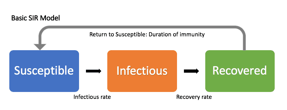
The SIR model we will look at today will split the population into 3 groups:

• S - Susceptible: Everyone who is able to catch the disease
• I - Infectious: Everyone who has the disease/can infect others
• R - Recovered/Removed: Those who have recovered or have been removed from the population

Using these groups, we will then establish how the population moves between them. We use a very useful fact about differential equations: they allow us to describe things that seem natural (how things change over time) in a mathematical way, and then by solving them we understand how this short term behaviour leads to long term consequences. So in essence, we dont need to create a function for how many people will get infected from scratch, instead we describe how they become infected and then solve. So we can visualise these compartments as follows:

We will study these compartments as fractions of the population:

Before we can introduce the models of how the population moves between these fractions, we first need to define $R_{0}$

The basic reproduction number, $\boldsymbol{R_{0}}$

$R_{0}$ can be thought of as "the expected number of cases directly generated by one case in a population where all individuals are susceptible to infection." 1 Technically once the epidemic is underway, we should be calling it $R_{e}$ (Effective reproductive number), but I am not feeling pedantic so we will stick with $R_{0}$. This function is quite important, because in essence it captures how actively the virus is spreading throughout the community. I say this because $R_{0}$ basically consists of:

where

$\boldsymbol{P_{\text{transmission}} \ =}$ Probability a sick person will infect a susceptible person if they meet.

$\boldsymbol{N_{\text{encounter}} \ = }$ Expected number of contacts between any two people within time $= \tau$

So clearly it is largely driven by the behavioural (how we act) and biological (how the disease works) characteristics of the epidemic.

It therefore makes sense to define $R_{0}$ in terms of the number of susceptible $s(t)$ and number of infected $i(t)$ at any given time $t$. E.g. when everyone is susceptible, you are more likely to infect someone.

It is also worth noting what the approximate range for $R_{0}$ is, and what the $R_{0}$ of other famous diseases are:

• COVID-19: $R_{0} \approx \text{3-6}$.

• Influenza: $R_{0} \approx \text{0.9-2}$.

• Measles: $R_{0} \approx \text{12-18}$.

• HIV: $R_{0} \approx \text{2-5}$.

• Ebola: $R_{0} \approx \text{1.5-2}$.

Some examples of what an $R_0$ function could be:

• $R_{0}(i, s)=4$ (constant throughout - most simple)
• $R_{0}(i, s)=4\left(1-9(1-s) s^{4}\right.$
• $R_{0}(i, s)=6(1.3+\cos (2 \pi s))^{1.9}$ (not covid realistic, but interesting)

Note we are only interested in $R_{0}$ over the range $0<s,i<1$, since this is the domain for the proportions of our population.

We can then introduce the differential equations we will use to model how the population moves between these compartments:

where:

• $\tau \ \approx$ time needed to "recover" from the infection.
• We also know from empirical evidence that $\tau \ \approx \ \text{2-4 weeks}$

It is always worth understanding what equations like these mean in simple language. Otherwise they don't mean too much. What we can wee above is that the rate of change from susceptible (i.e. how people are leaving the susceptible compartment or $\large \frac{d s(t)}{dt}$) multiplied by $\tau$ is defined by some function. This function consists of the reproduction function at that point ($R_0$), the susceptible fraction at that point ($s(t)$), and the infectious fraction at that point ($i(t)$). When I first saw this equation I was slightly confused as to why we were multiplying by $\tau$, and have since come to understand that $\tau$ represents our time frame. I.e. the change in $s(t)$ over a $\tau$ period is equal to $- R_{0}\, s(t)\, i(t)$.

As you can see, the equations are symmetric, the fractions of the population that leaves $S$ enters $I$. We can then add the equations together and we get:

This agrees with our definition for the proportion of population entering the "recovered" compartment over 1 time interval.

This made all the equations click for me and convinced me that even though it is not the most sophisticated models, they are useful in understanding how the dynamics behave since:

$\ 1 \ time \ interval \approx \tau \ \approx$ time needed to "recover" from the infection.

Therefore, if in time interval 1 there were 10% of the population in $I$, as we go to time interval 2, that 10% leaves $S+I$ and enters $R$.

Recovery Function

There is one last piece of maths we need to model this effectively. In order to understand how many people are in the $i(t)$ and $s(t)$ compartments, we need to be able to establish the proportion of people in the recovery compartment $r(t)$. It is also easier if we can do this in terms of $s$, as opposed to $t$. Hence we do:

In simple terms, this represents the change $r$ as we move forward in time. However, since $s$ begins at 1 and decreases to $0$, we thus must work backward in time to calculate the sum. We can thus flip the sign and integrate to calculate the given number of recovered cases for any $s$:

This step is a little confusing - but we need this recovery function to be able to compute the proportion of the population which is infected when the virus peaks, and the proportion of the population susceptible after the first wave finishes. The key equation to remember here is:

From this equation we are able to work out the maximum number of infections as well as the final susceptible number:

Final susceptible population

If we want to find which proportion of the population is still susceptible when the infections are gone, we need to solve:

Since this implies 0 proportion of the population is infected. We can use Newtons method to solve for $i(s) = 0$, to ensure that we are able to solve for any $R_{0}$ function.

Maximum infections

We can find the maximum number of infections by solving for where $i'(s) = 0$. This corresponds to the peak of the infection curve:

Therefore, we have to solve

Using Newtons method.

Conclusion

Now we have built a solid foundation so we can understand how different $R_{0}$ functions lead to different outcomes. And since $R_{0}$ functions represent policy choices, we can understand which policy choices we need to take. Off to Part 2 we go!

Part 2 - Modelling outcomes and policy choices

In Part 1, we became familiar with SIR models which places the population into 3 bins:

• Susceptible
• Infectious
• Removed/Recovered

We also created some mathematics which allows us to study how the population moves between these sections, with one of the big factors being how the function, $R_{0}$, looks at certain points in time.

Now we can begin to visualise and understand how our actions affect the spread of the virus. Unfortunately I will be unable to share all of the code publicly, as this post was originally inspired by a University assignment which will put me at risk of being copied. However, if you are interested, email me @ tiaanstals98@gmail.com!

Case 1 - what if we did nothing?

And here, I mean like nothing nothing. No wearing masks, no travel restrictions - we simply continued working and living as if nothing was going on. A recent report published by the Australian Department of Health concluded the $R_{0}$ for COVID-19 $\approx 3.3$, which we can use as our baseline (when everyone is susceptible). Its worth noting there is no consensus on the $R_0$ of COVID-19 and there are only estimates at this stage.

So the problem becomes, we have some research which indicates the $R_0$ of COVID-19 to be approximately $3.3$, but the key definition states that this is in a completely susceptible population. However as more people become infected and then no longer susceptible, the entire population is no longer able to catch the disease. There is no clear literature on exactly how as the susceptible proportion of the population changes, $R_0$ changes. For simplicity sake, I am going to treat $R_0$ as an expected value. Given some proportion that is still susceptible $s$, how many secondary cases can we expect from $1$ infectious person? I am going to model this quite simply:

Hence, our $R_{0}$ function would be a factor of the base $R_0$ (3.3) multiplied by the proportion of the population still susceptible. If we visualise what this looks like over our susceptible domain we see the following:

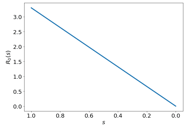
As you can see, the number of secondary cases we expect an infectious case to generate slowly decreases as the proportion of the population which is still susceptible decreases. To me this makes intuitive sense, if everyone is sick, you can't expect to infect the same number of people as when no one was sick. Now that we understand the construction of our $R_0$, we can begin to analyse how this will affect the disease dynamics.

Solving for case 1

Using this $R_{0}$ function, we can then solve the ODE's using a beautiful open source library known as scipy if given some initial conditions. Doing so we see the following results:

• Intial conditions: $i_0 = 0.0000001$ (i.e. initially about 2 people infected if we use Australia), $s_0 = 1$ (everyone is susceptible)
• Peak infections: At the peak, 20.21% of the population is in the infectious bin, and 55.05% is still susceptible. Huge numbers!
• Final conditions: 30.03% of the population is still susceptible! 69.69% of the population either recovered or was "removed" from the population.
• Here is the plot:

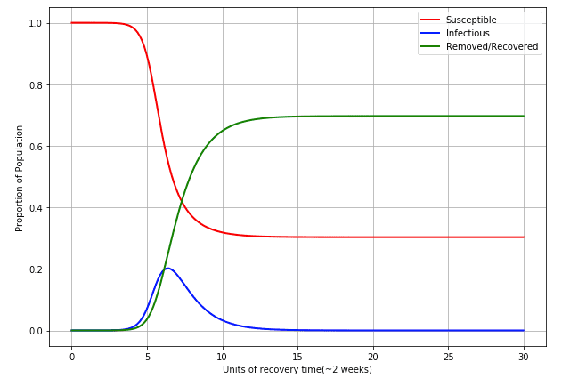
The numbers here are fairly self evident that this would not be a good outcome. The most worrying factor here is the peak of the infectious proportion of the population. If 20% of Australia were to get the virus at the same time, our medical systems would be completely overwhelmed, and the ~70% of people in the "recovered/removed" section would probably be more "removed" removed than we would like. I haven't made my recovery function a factor if the infected proportion at any given time, but in real life I expect this to be correlated. If everyone is sick at the same time, more people will be "removed".

A few studies have tried to estimate the Case Fatality Rate (CFR) - the number of fatalities/number of cases. A widely accepted study by The Lancet Medical Journal 2 found the following estimates for the CFR of COVID-19:

• 0·32% 0.27-0.38 in those aged <60 years
• 6·4% 5.7-7.2 in those aged ≥60 years
• Overall 1.38%

We can see here that if 1.38% of people who got the virus died, and 70% of Australia's 25M people got the virus, we could have:

$0.0138 \times 0.7 \times 25,000,000 \approx 241,499 \ fatalaties$

Of course this is under extremely simplified conditions, but its interesting to look at. As we now compare to different policy responses we also see how this compares relatively. We also assumed the proportion of $R_{0}$ that is generated by how people act to be constant. This means no intervention at all, so this isn't an overly realistic response from any country, however it is worth considering as a baseline.

Case 2 - Sweden Style

Sweden choose to not impose any significant restrictions on it's citizens instead asking them to voluntarily maintain social distancing protocols. Although the economic burden of such a strategy is much lower, Sweden has reported around 321 cases per 100,000 people (as of May 22). The only countries with higher cases per capita rates is Spain, Belgium, the US, the UK and Italy. This is an interesting strategy, and probably reflects what the "post-covid" world will be like. There may be no strict restrictions, but there will be a good amount of "voluntary" social distancing, hesitation, wearing masks etc. until we have a vaccine.

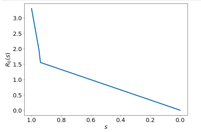
In terms of how this would look as an $R_{0}$ function, we might expect that at the start before anyone is aware of the virus, it begins at 3.3 and then, as well as being a function of $s$, the part of $R_0$ that is determined by human behaviour may also decrease to reflect "voluntary social distancing". Remember from our definition of $R_0$:

$R_0 \approx \text{probability of transmission} \times$ the number of encounters an infectious person has

So we know as $s$ decrease the number of encounters with susceptible people decrease. We reflect this with our above "do nothing" function, but now we need to incorporate some maths which reflects a reduction in the probability of transmission.

Another study I read in The Lancet 3 found that strict social distancing measures could achieve a reduction in $R_{0}$ of up to 60%. Since in this case of Sweden, the social distancing won't be incredibly "strict" I will make the assumption that Sweden style social distancing will only lead to about a 50% reduction in the original $R_{0} = 3.3$ number. Hence we can establish an $R_{0}$ function:

Which essentially means $R_{0}$ quickly decreases to $1.65 \cdot s$ as people become more familiar with social distancing, and stays there until there is heard immunity. We can visualise what $R_{0}$ would move like as $s$ changes:

Using this $R_0$ function, we can now solve for our predicted outcomes.

Solving for case 2

We have had to make a few assumptions to figure out what this $R_0$ function might look like. Its not black and white which we need to remember but now we can see how these assumptions affect our model.

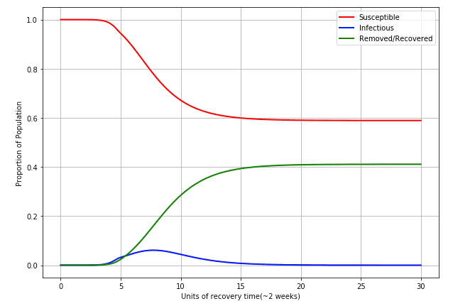
Here are some of the results:

• Intial conditions: $i_0 = 0.0000001$ (i.e. initially 2 people infected), $s_0 = 1$ (everyone is susceptible)
• Peak infections: At the peak, 6.09% of the population is in the infectious bin, 77.85% is still susceptible.
• Final conditions: 58.9% of the population is still susceptible! 41.09% of the population either recovered or was "removed" from the population.
• Here is the plot:

As we can see here doing something is certainly better than doing nothing at all. Empirical evidence by a study 4 from the University of Auckland shows the effective $R_0$ in Sweden hovering between 1-2, but mostly tending back to about 1. I would estimate the $R_0$ constructed above with 1.65 is therefore on the high side, and it may be worth reflecting an $R_0$ between 1.2-1.4

Case 3 - Australia

For my last case I am going to be considering a situation similar to what is happening in Australia. We will begin with a relatively high $R_0$, which will then drop sharply to reflect strict social isolation and social distancing policies. The $R_0$ will then remain low for some time, before gradually increasing again, to simulate the easing of restrictions. In order to reflect these conditions, I will also need to consider time as a variable.

Before we can formulate a complete $R_0$ function, we need to do some investigation. Firstly, from the data Australia has had about 7000 cases. This since this is $\frac{7000}{25000000} = 0.00028$, we know that from $s = 1$ to $s = 1 - 0.00028 = 0.99972$ Australia's actual $R_0$ has dropped from 3.3 to < 1 (here assumed to be 0.9). We also know that as the economy opens up, this number will likely go back up again. So firstly, we can model one part of the $R_0$ function, that by $s = 0.99972$, $R_0$ should be less than 1. So we can begin constructing our equation:

This reflects how Australia's real $R_0$ number has dropped by the time our susceptible fraction is equal to 0.99972. So far we have the following $R_0$:

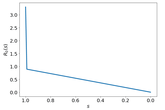
Now what we must consider is the time element. Essentially what we are doing in Australia is that we have reduced $R_0$ down to this level, and it has stayed there for about a month and a half. As I am writing this, it is June 1 and Australia has re-opened a lot of establishments including schools, pubs/restaurants and some other businesses. It is very hard to predict how this will affect the $R_0$.

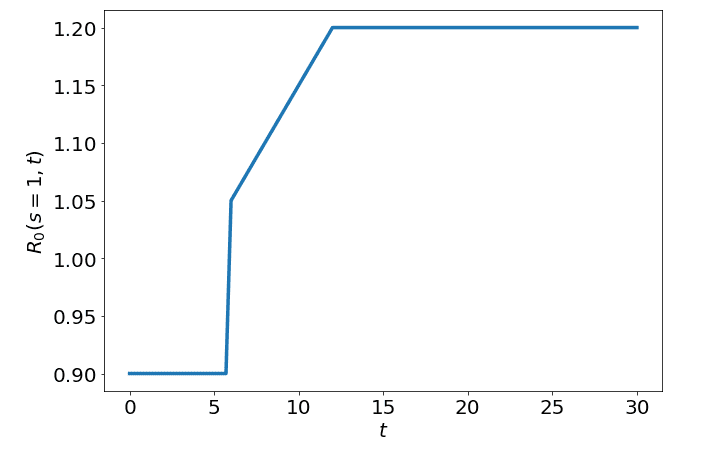
So here I am going to have to make a few assumptions. I am doing to be slightly pessimistic, and say that for every 5 infectious cases, on average we will see those 5 cases create 6 secondary cases. This will give us a baseline $R_0$ of 1.2. So by the time the economy is fully opened up this is what we will see. Assuming no vaccine. We must also then work out how we place this time wise. Google Data tells me the first case was on January 25th, so essentially this will be $t = 0$. We are also working in recovery time units (lets say 3 weeks), so from the first case to now it has been about 18 weeks, or 6 time units.

Hence, from t = 6 - 12, we will see the $R_0$ gradually increase to 1.2. Hence we then need to modify our $R_0$ function as follows:

$R_{0}= \begin{cases} 3.3\cdot\ s -\left(3.3\cdot0.9\right)\cdot\left(\frac{\left(1-s\right)}{0.07}\right) , & \text{for } 1\leq s\leq 0.99972\\ s \cdot \left(3.3- (0.5 \cdot 3.3)\right) , & \text{for } 0.99972\leq s\leq 0 \ , \ 0\le t\leq 6\\ s \cdot \left(3.3- (0.5 \cdot 3.3)\right) \ + (\frac{t}{12} \cdot 0.3) , & \text{for } 0.99972\leq s\leq 0 \ , \ 6\leq t\leq 12\\ s \cdot \left(3.3- (0.5 \cdot 3.3)\right) \ + 0.3 , & \text{for } 0.99972\leq s\leq 0 \ , \ 6\leq t\leq 12\\ \end{cases}$

So if we consider how $R_0$ looks as we move forward in time (ignoring s) we would see this:

We can also plot both $s$ and $t$ on separate axis and we would see the following:

Before attempting to solve this model, I was completely unsure as to what was going to happen! It was exciting in a nerd like way. So here come the results:

Using the function above exactly as described, we reach a peak percentage of infections of... unclear. This is a rather interesting case. Using the same timescales as above, we find the following chart:

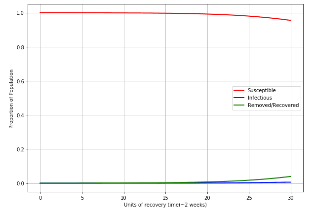
What is interesting here, is even though we have no definite peak within the first 30 $\times$ 3 weeks = ~1.8 years, the virus is still growing at the end of the time period, and the max infections occur then with 0.59% of the population being infected at that point and 95.45% still being susceptible (i.e. in 4 years, ~5% of the population got the virus)

So what happens if we extrapolate further?

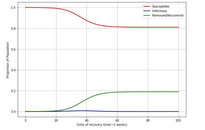
If we extrapolate over 300 weeks, or ~6 years, we see that about 20% of the population get the disease at one point or another. This is assuming a vaccine is not developed, and we have an $R_0$ of approximately 1.2. It is rather interesting to look at it from this point of view. Of course this isn't a very sophisticated model, it does reflect some aspect of reality. Until there is a vaccine, the population will keep getting the virus. It will be part of the new norm of life. A recent study by The University of Sydney shows that lower humidity could lead to a significant increase in the number of cases.

So the virus can very easily become a cyclical type disease, which spikes in winter time. One thing to consider is that the virus may also mutate, like the flu. This means the idea of a vaccine is more difficult, and its something we will need to get every year.

Thanks

If you made it this far, congrats! I certainly think I would have struggled. I hope you learnt something new about COVID-19 and you are a little more informed for reading this post.

Footnotes

1 Fraser, Christophe; Donnelly, Christl A.; Cauchemez, Simon; Hanage, William P.; Van Kerkhove, Maria D.; Hollingsworth, T. Déirdre; Griffin, Jamie; Baggaley, Rebecca F.; Jenkins, Helen E.; Lyons, Emily J.; Jombart, Thibaut (June 19, 2009). "Pandemic Potential of a Strain of Influenza A (H1N1): Early Findings". Science. 324 (5934): 1557–1561. Bibcode:2009Sci...324.1557F. doi:10.1126/science.1176062. ISSN 0036-8075. PMC 3735127. PMID 19433588

2 Verity, R., Okell, L., Dorigatti, I., Winskill, P., Whittaker, C., & Imai, N. et al. (2020). Estimates of the severity of coronavirus disease 2019: a model-based analysis. The Lancet Infectious Diseases, 20(6), 669-677. doi:10.1016/s1473-3099(20)30243-7

3 (2020). Thelancet.com. Retrieved 31 May 2020, from https://www.thelancet.com/pdfs/journals/lancet/PIIS0140-6736(20)30567-5.pdf

4 6 countries, 6 curves: how nations that moved fast against COVID-19 avoided disaster. (2020). The Conversation. Retrieved 1 June 2020, from https://theconversation.com/6-countries-6-curves-how-nations-that-moved-fast-against-covid-19-avoided-disaster-137333